Matrix decomposition, the basis for ML

February 10, 2024 - 11 minutes

Summary

1. Some Algebra basics
2. EigenValue Decomposition
3. Spectral Decomposition
4. SVD decomposition

In the field of Machine Learning, Algebra serves as the backbone of our work. In this article, we’ll explore key Algebraic concepts essential to understand the underlying principles of the Python libraries commonly used in our ML projects. Let’s delve deeper into this fundamental Algebra and its applications in ML.

Some Algebra basics

First of all, it is necessary to introduce some concepts that are foundamental to understand the concepts of SVD, the basic ideas are:

• Diagonal matric implies shrink or stretch of the orignal matrix
• Orthogonal matrix implies rotation of the original matrix

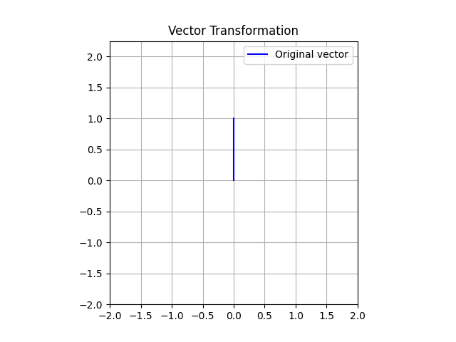
Here we can see a graphical representation. Let’s consconsider we want to verify the effects on a simple vector $v=[ 0\; 1 ]$, here there is a plot of this vector:

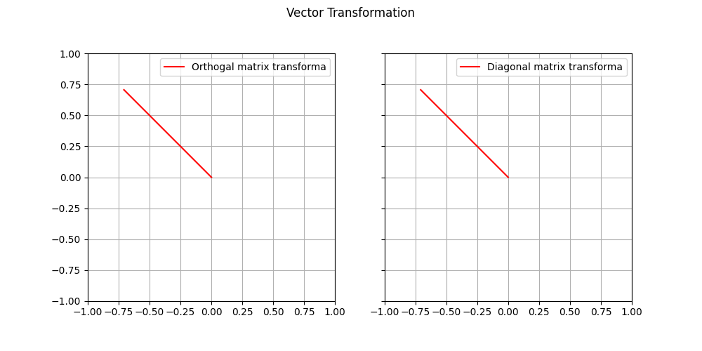
Now, let’s calculate the matrix multiplication of $v$ with both an orthogonal and a diagonal matrix. I consider $Q=\begin{bmatrix} 0.707 & 0.707 \\ -0.707 & 0.707 \end{bmatrix}$ as orthogonal matrix and the matrix $D=\begin{bmatrix} 0.5 & 0 \\ 0 & 2 \end{bmatrix}$ as a diagonal matrix. Here we can see the result:

Eigenvectors and eigenvalues, in short

Before go into detail in the matrix-decomp, it’s essential to clearly define the geometric meanings of eigenvectors and eigenvalues.

Eigenvectors of a square matrix are special non-zero vectors that, when multiplied by the matrix, yield a scaled version of themselves. They have a unique property: their direction remains unchanged even under various transformations of the matrix. This inherent stability makes them pivotal, since eigenvectors represent distinct and unchanging characteristics of the matrix. Moreover, the associated eigenvalues play a critical role because they define how the matrix is scaled along the directions defined by eigenvectors. As my professor said, “eigenvalues are particular signs of the matrix”.

More formally, eigenvalues are those values that allow satisfying the relation:

where $\lambda$ is every eigenvalues of the matrix $A$ and $I$ is the identity matrix.

Some properties of eigenvalues are:

• Every square matrix has at least one eigenvalue, which may be real or complex
• The sum of all eigenvalues of a matrix is equal to the sum of its diagonal elements (trace of the matrix)
• The product of all eigenvalues equals the determinant of the matrix
• If A is square and $\sigma(A)$ the set of eigenvalues of A, then $\sigma(A)=\sigma(A^T)$
• If a matrix has all eigenvalues $>0$ then the matrix is positive definite, otherwise if all eigenvalues are $<0$ the matrix is negative definite
• Eigenvalues remain unchanged under similarity transformations, meaning if A and B are similar matrices they share the same eigenvalues. (Two matrices A and B are similar if $B=P^{-1}AP$ where P is the matrix acting as the change of basis matrix)

Formally, we can also define the relation between eigenvectors and eigenvalues:

where $v$ is the eigenvector associated to the eigenvalue $\lambda$.

Some properties of eigenvectors are:

• Eigenvectors corresponding to different eigenvalues are linearly independent
• The eigenvectors corresponding to an eigenvalue $\lambda$ form a subspace called the eigenspace or null space of $\lambda$
• Similar matrices share the same eigenvectors, though they may have different eigenvalues
• Eigenvectors corresponding to distinct eigenvalues of a symmetric matrix are orthogonal to each other

Overall, the main geometrical idea behind these two concepts is:

The eigenvector points in a direction in which the vector is scaled by transformation, and the eigenvalue is the factor by which the vector is scaled.

Matrix composition and decomposition

We need to define two main concepts:

• Matrix composition: in simple words, a matrix composition is the result of the product between matrices that provides a new matrix, composed by the initial matrices. This is very easy to calculate.
• Matrix decomposition: this is the opposite of composition. It is also called matrix factorization and it is a factorization of a matrix into a product of more matrices. The main idea is to find the matrices which multiplicated provides as a result the initial matrix. This is very challenging in Algebra, but it is super important. There are many different kind of decomposition and they are used in different contextes and assumptions. At the end of this section we’ll see an important decomposition that will be helpful for the SVD decomposition.

Before go in deep, I want to show two very similar matrix-decomp:

• EigenValue Decomposition (EVD)
• Spectral Decomposition

EigenValue Decomposition (EVD)

The EVD is a very simple decomposition, but it requires one assumption: the matrix $A$ must to be a $n\times n$, so the matrix has to be square. This is the formulation:

where $V$ is the matrix of the eigenvectors of $A$ and $\Lambda$ is the diagonal matrix of the eigenvalues of $V$.

This is easy to see since if $v$ is an eigenvector (column vector) of $V$:

The linearly independent eigenvectors associated with eigenvalues different of 0, form the basis of the column space of $A$. The linearly independent eigenvectors associated with eigenvalues equal to 0, form the basis of the null space of $A$.

Spectral Decomposition

Symmetric matrix

The symmetric matrix, as you probably know, is a matrix where the values at the specular postion compared to the diagonal are the same. More formally it is defined as:

Where $s$ is any values of the symmetric matrix $S$. Moreover, a symmetrix matrix is always a square matrix, and it is equal to its transpose matrix.

An other important property of symmetric matrices are that the matrix of eigenvectors (which contains on the columns the eigenvectors of matris) is always orthogonal. This property is very important, let’s see why in the next paragraph.

Orthogonal matrix effects

Let’s consider an orthogonal matrix. We know that a matrix mutliplication with an orthogonal matrix produces a rotation, so if we perform the multiplication with the inverse of the orthogonal matrix, we obtain a rotation in the opposite direction. But we know also that the inverse of an orthogonal matrix is equal to its transpose, $Q^{-1}=Q^T$. Therefore, the multiplication of a matrix with the transpose of an orthogonal matrix, produces a rotation in the opposite direction.

To be more clear, I want to show you a plot that proves what we just said. The initial vectors is still $v$ and the orthogonal matrix is $Q$ (that we defined above).

As we can see, the result of the rotation is the same for both inverse and transpose of the orthogonal matrix. Interesting, don’t you think?

Spectral Decomposition, formalization

Now that we are on the same page, we can start with the Spectral Decomposition. This decomposition is applicable only on symmetric matrices, in fact in these kind of matrix the eigenvectors are orthogonal. This implies that exist always an orthogonal matrix which rotates the basis to align the eigenvectors and the inverse of that matrix (equal to the transpose, since it is orthogonal) which would rotate the eigenvectors to align with the basis.

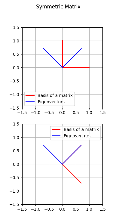
In the follwing picture we can see an example on how the basis is align with the eigenvectors.

For the latter assumptions, we can define the Spectral Decomposition as follows:

where $Q$ is the orthogonal matrix composed by the eigenvectors of the symmetric matrix $S$, and $\Lambda$ is the diagonal matrix composed by the eigenvalues of the matrix $S$.

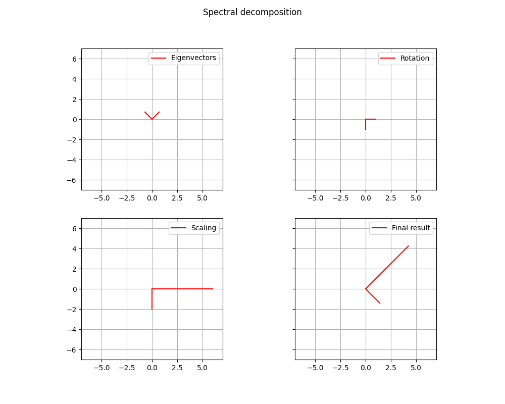
The significant of this descomposition is incredible. The orthoganl matrix $Q$ represents the rotation of the decomposition, while the matrix $\Lambda$ represents the stretch of the decomposition. As result we have, first the rotation of the eigenvectors due to the orthogonal matrix $Q$, then the scaling due to the diagonal matrix $\Lambda$, eventually we have the rotation in the opposite direction due to the transpose of the orthogonal matrix $Q^T$.

The Spectral Decomposition of the example is the following:

We can see the result in the graph.

SVD decomposition

This is one of the most important concepts in Algebra, especially for its applications in Data Science and Machine Learning. We can find this decomposition in PCA, low-rank approximation, TLS minumum, pseduinverse, and etc.

First, we have to define some aspects. In general the matrices are not symmetric and square, but they are rectangular. How this kind of matrix can help us? An example is the trnsformation of a matrix or a vector from a dimension to another. Let’s take an example.

We have a vector $v=\begin{bmatrix} 1 & 2 & 0\end{bmatrix}$ of dimension 3 and we want to erase a dimension and take it to dimension 2. In order to do this we can use a rectangular matrix as here:

# Always remember that the result has dimensions: (#row_first × #columns_second) = (m × n)

The rectangular matrix that we used above, it is the identity matrix of dimension $2\times 3$. This kind of matrix allows to erase one dimension and lead a vector $v \in \mathbb{R}^3$ to the dimension $\mathbb{R}^2$. This matrix, basically, remove the value of z-axis. Simple but effective.

On the other hand, we can use that matrix as a adder of dimension. You’ll wonder how. Well, it is rather easy. You need just to transpose that matrix and the game is done. Let’s take and example:

We can apply the same reasoning on the matrices. Here we have an example with a diagonal matrix:

In this case the matrix changed from a dimension $2\times 2$ to a dimension $2\times 3$, so from $\mathbb{R}^2$ to $\mathbb{R}^3$$.

On the same way we can define the matrix as a decomposition of the previous:

where

• the matrix $\begin{bmatrix}1 & 0 & 0 \\0 & 1 & 0\end{bmatrix}$ increase the dimension
• the diagonal matrix stretch the matrix along the axes, in this case multiplying the x-axis by a factor of 3, the y-axis by a factor 4.

Ok, but did we talk about symmetric matrices?

Good question. In the previous section, we discussed about symmetric matrices, and they are always square matrix. But in reality, most of matrices they are used in practice, are not square. On the contrary, having a square and symmetric matrix is fluke. So there is a techinque that allows to get a square matrix even if we are working on a rectangular matrix, let’s see how with an example.

In this case we take a matrix $3\times 2$:

Now, we multiplicate this matrix by its transpose, so $AA^T$:

The result is surprising: the matrix is a square and symmetric matrix!

Now we do the same but multiplying the transpose by the original matrix, so $A^TA$:

Also in this case the result is a symmetric matrix, great!

This is not a coincidence, every time we multiply the matrix by its transpose or the transpose by the original matrix, we get 2 symmetric matrices which come from a rectangular matrix.

Now we can get the eigenvectors of every matrix:

• The eigenvectors of $A^TA$ are called right singular vectors
• The eigenvectors of $AA^T$ are called left singular vectors

All these singular vectors are different and are all related to the original rectangular matrix. This will help us to explain the SVD.

Important to note that both new matrices are semi positive definite. This is a brief proof:

Let $v$ a non-zero vector:

The result represent the Euclidean norm, that is always greater or equal to zero. We can apply the same proof for $AA^T$, the result is the same.

Singular values

Since that the matrices are semi positive definite, every $\lambda_i\geq 0$. Now, if we order all the eigenvalues of $AA^T$ and $A^TA$ from the highest to the lowest, we discover an intersting coincidence. All the eigenvalues found are equal for both matrices, so $\lambda_{i,A^TA} = \lambda_{i,AA^T}$, and those eigenvalues that are different, are equal to 0.

Let’s do an example. Consider $A=\begin{bmatrix}3 & 2 & 2\\2&3&-2\end{bmatrix}$ and then we calculate

• $AA^T = \begin{bmatrix}17 & 8\\8 & 17\end{bmatrix}$ where the eigenvalues are: $25$ and $9$
• $A^TA = \begin{bmatrix}13 & 12 & 2\\12&13&-2\\2 & -2 & 8\end{bmatrix}$ where the eigenvalues are: $25$, $9$ and $0$

From these eigenvalues we can calculate new values, as follows:

This values are very important for SVD, they are the singular values of the matrix $A$. In this case the values are $\sigma_1 = 5$ and $\sigma_2 = 3$.

SVD, formalization

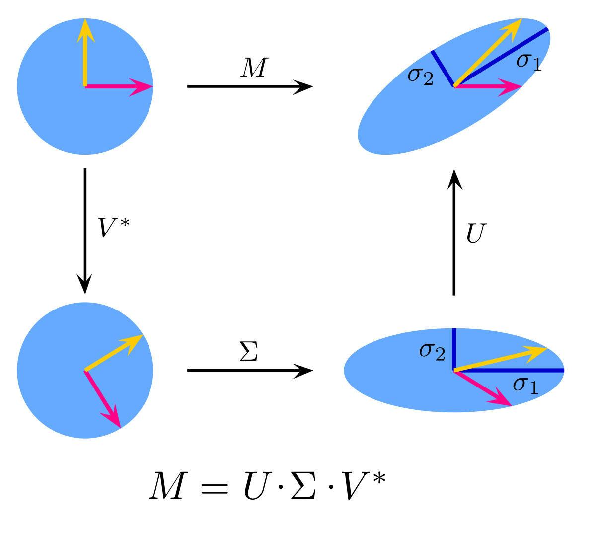
Now we have all the elements that we need to formalize the SVD decomposition. As we have already said, the SVD decompostion is applicable to every rectangular matrix, and it can be decomposed as it follows:

where $U$ is the orthogonal matrix of the singular vectors of matrix $AA^T$ (left singular vectors), so every column contains a singular vector. $V$ is the orthogonal matrix of the singular vectors of matrix $A^TA$ (right singular vectors), but in this case every singular vector is on the row, since it is transposed. $\Sigma$ is the rectangular diagonal matrix that contains on the diagonal every singular value from the highest to the lowest.

Now, let’s take as example the matrix $A=\begin{bmatrix}3 & 2 & 2\\2&3&-2\end{bmatrix}$ that we used before. I want to show what happens when we calculate the original matrix, starting from the decomposition. Initially, we start with $V^T$. This matrix operates a rotation in the same dimension on which it is, such that the right singular vectors return to the standard basis. In simpler terms, $V^T$ adjusts the orientation of the output space so that the transformed vectors align with the original axes (standard basis). In this example $V^T=\begin{bmatrix} -0.7 & -0.7 \\ -0.7 & 0.7 \end{bmatrix}$.

Now, we have to consider two cases, based on the dimension of the matrix $A$:

• If $m<n$, if the number of rows is lower than the number of columns

In this case the action of $\Sigma$ on the matrix $V^T$ consists to erase a dimension. As we saw before, we can consider $\Sigma$ as a rectangular diagonal matrix in this form:

Notice that by the decomposition of the matrix, we can find the “rectangular square matrix” that we described above. This is very significant, since this show that the $\Sigma$ with these dimensions will erease a dimension of $V^T$. In addition it is composed also by a diagonal matrix that will rescale the matrix on x-axis and y-axis based on the singular values 5 and 3, respectively.

• If $m>n$, if the nummber of rows is greater than the number of columns

On the contrary, if $\Sigma$ had these dimensions, it would add a dimension to $V^T$. The reasoning is similar on what we did for the other case, so by the decomposition we would have found the matrix $\begin{bmatrix} 1 & 0 \\ 0 & 1 \\ 0 & 0 \end{bmatrix}$ that means to add a dimension.

Eventually, we multiply the matrix $\Sigma V^T$ calculated so far with $U$. In this case there is another rotation since the matrix $U$ is orthogonal. This matrix rotates the standard basis to align with the left singular vectors.

Here we are! We complete the transformation, that is exaclty the same as $A$ matrix. In the following picture we can see the result.

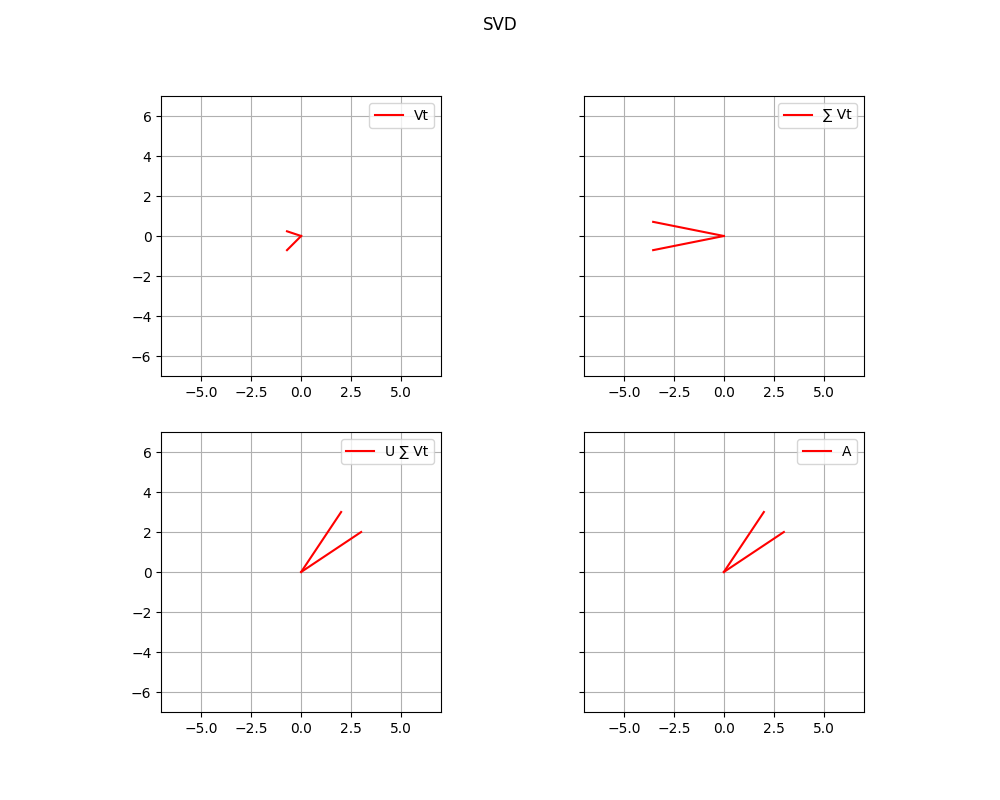
In general, we can define every transformation operated by each matrix of the decomposition as we can see in the following picture:

We can see that the vectors change their direction because of the matrices $V$ and $U$, which are the matrices of the singular vectors, and because of the matrix $\Sigma$ the vectors are stretched. The final result is a new view of the same matrix.

We finished!

By those decomposition it is possible to have a new view of the problem. Imagine these matrices as vast collections of data. Having this new viewpoint, especially with SVD, proves highly beneficial. This separation allows us to isolate and analyze each component independently, which can be helpful to understand the individual contributions of rotation and scaling to the overall transformation of the data. Additionally in other contexts, every matrix describes how the original basis vectors are rotated in the transformed space, revealing patterns and relationships that may not be evident in the original data. This newfound understanding has several applications, from denoising to compression, and even aiding in predictive analysis.

Thanks for reading!😃