Multi linear regression for calibration

March 10, 2024 - 6 minutes

Summary

1. What is the experiment?
2. Multi linear regression

What is this experiment?

In this experiment we are going to see a very used technique to reconstruct a reference dataset, based on the combination of different variables. I am talking about regression. This is a very famous technique applied in data analysis.

The scenario is the following. We need to estimate the level of $O_3$ in the air of a specific zone. In this zone there are few reference stations that are able to provide high trustable data, but we need to be more accurate. We need to increase the number of station, but it is not possible have available several reference station that measure those data, because they are more difficult to manage and maintain, so the costs are higher. The solution is to place on the specific area several small and cheap device that are able to measure the data. Despite we get an high benefits in terms of costs, however these devices are not so trustable. In addition, they read the $O_3$ values with another unit of measure. These devices have some more features, in fact, they can also read temperature and humidity in the air. We want to use these characteristics in our advantage.

At the end of the measurements we will have two dataset:

• Reference dataset: composed by the reliable data of $O_3$ and with $\mu gr/m^3$ as unit of measure
• Sensors dataset:
  • $O_3$ data: the dataset of the ozone in the air measured in $k\Omega$.
  • Temperature: the dataset of the temperature measured in °C.
  • Humidity: the dataset of the humidity in the air measured in %.

I want to compare only the $O_3$ data of both dataset, in the following picture.

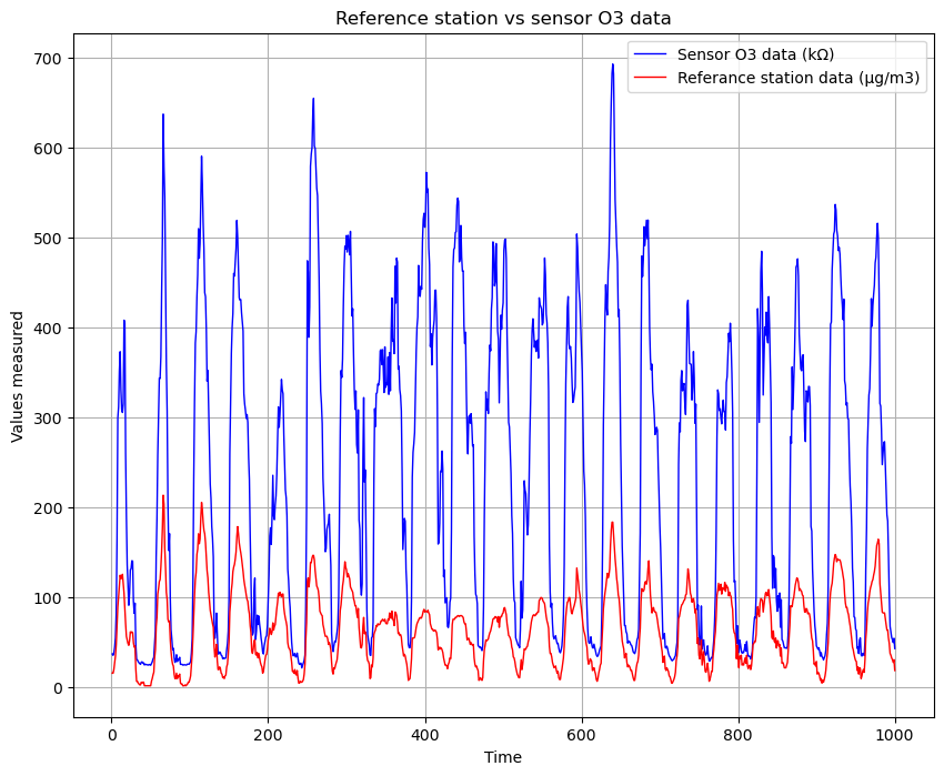
We can notice that the difference is evident.

Now, we want to compare every sensor dataset with the reference dataset. This is not possible with the current dataset, because every set has a different unit of measure. The solution is the normalization of the data. In this way we obtain in every set a mean equal to 0 and the variation equal to 1.

# I did the same operation in the last post. Check it!

For the normalization with respect to the mean and standard deviation, we calculate the mean of each dataset and the standard deviation. This is very easy in Python thanks to the NumPy library that provides useful functions. Once get these values, we can normalize using the following formula:

where $\bar{x}_{value_i}$ is every new value that will compose the dataset normalized.

The code that I implemented to normalize the data, is the following:

def normalization(dataset):
    mean = np.mean(dataset)
    sd = np.std(dataset)
    normal_dataset = []
    index = 0
    for index in range(len(dataset)):
        value = dataset[index]
        value = (value - mean)/np.sqrt(sd**2)
        normal_dataset.append(value)

Thanks to the normalization it is possible to compare every dataset with reference dataset. Let’s see some results. The first plot that I want to show represents the relation between the $O_3$ read by the sensors and the $O_3$ read by the reference dataset.

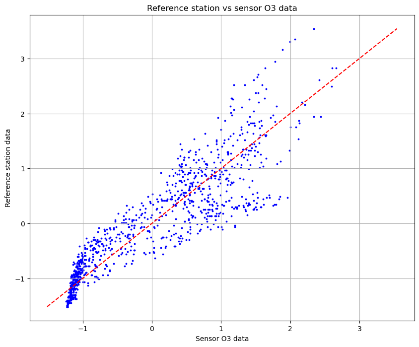
From the plot we can notice that there is a bit of correlation, even though the more the values are high, the more the distance increases. There is something to fix.

In the next plot, we can see the relation between the temperature and the $O_3$ read by the reference station.

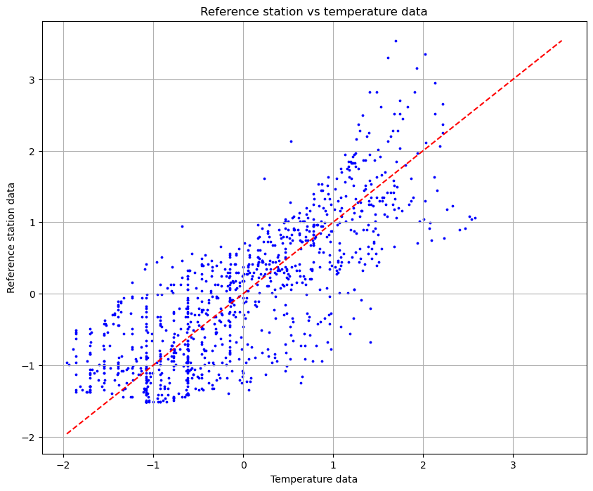
From the plot we can see that there is a slight correlation but the variation is too high. However, the temperature data can help the regression to achieve a better approximation.

Now, we can see the correlation between the humidity and the reference station, in the next plot.

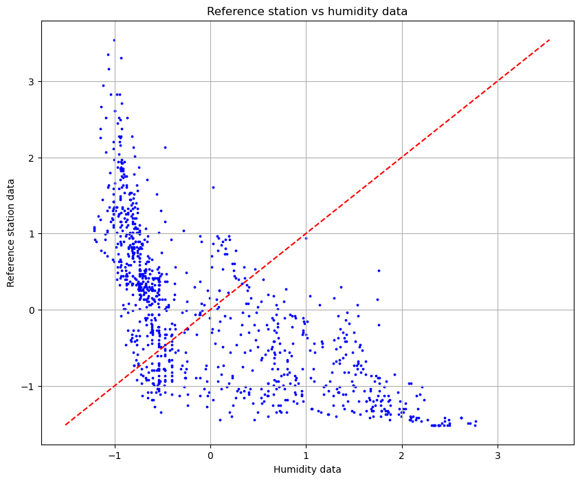
We can notice that there is a very high variation and the dots are very far from the line of perfect correlation. By this we can say that this data is not very relevant for the calibration. We will include this dataset in the regression to see what will happen.

# Notice that the oblique line represents y=x function, which is the perfect correlation.

Multi linear regression

Now, we can start with the regression. In data science, regression refers to a statistical method used to model the relationship between one or more independent variables and a dependent variable. The goal of our regression analysis is to understand how the $O_3$, temperature and humidity measured by the sensors can predict the true values of the $O_3$ measured by the reference stations. This technique is commonly used for forecasting, hypothesis testing, and understanding the strength of relation between variables.

More specifically, in our case, we implement the multi linear regression, since we have available more than one variable to calibrate the sensors. The model that we want to build is the following:

The model in multi linear regression is composed by different parameters $\theta$ that change the value based on the relevance that every component ($O_3$, temperature and humidity) has.

For build the model, first of all, I need to define four dataset:

• X training set: it is the dataset that allows to train the model. The data are taken randomly from the sensors data. For the modeling I use 70% of the total dataset.
• X test set: it is the dataset that allows us to test the model after the training. The data are taken randomly from the sensors data. I use the remaining 30% of the whole dataset.
• Y training set: it is the dataset used for the training. Every time the model tests a new value using the X training set, then it is compared to the Y training set in order to check if the result is close or not. If not the model is correct and proceed with the next value to test. Also in this case, 70% is used.The data are taken randomly from the reference stations data.
• Y test set: it is used to validate the model in the testing phase. The data are taken randomly from the reference station data. This data represents 30% of the whole dataset. Notice that every value taken from the dataset is picked randomly in order to train and test better the model, and the datasets that I used contain the normalized data.

The code is not so complicated, since NumPy and scikit-learn are very useful libraries to use in these contextes.

import numpy as np  
from sklearn.linear_model import LinearRegression
from sklearn.model_selection import train_test_split

This is the code used to calculate the new function thanks to the regression:

# Function to calculate the root mean square error (RMSE) between two arrays
def calculate_rmse(X, Y):
    difference = X - Y
    squared_diff = difference**2
    mean_square_diff = np.mean(squared_diff)
    rmse = np.sqrt(mean_square_diff)
    print(f"RMSE = {rmse}")
    return rmse


# Create a training set by zipping and converting to list the normal_o3_dataset, normal_temp_dataset, and normal_hum_dataset
normal_data_training_set = [list(a) for a in zip(normal_o3_dataset, normal_temp_dataset, normal_hum_dataset)]

# Split the dataset into training and testing sets
y_train, y_test, x_train, x_test = train_test_split(refSt_dataset, normal_data_training_set, test_size=0.3, random_state=42)

# Convert the training sets to numpy arrays
x = np.array(x_train)
y = np.array(y_train)

# Initialize a Linear Regression model with fit_intercept set to True
model = LinearRegression(fit_intercept=True)

# Fit the model with the training data
model.fit(x, y)

# Calculate the coefficient of determination (R squared) of the prediction
r_sq = model.score(x, y)

# Print the intercept (theta_0) and coefficients (theta_1, theta_2, theta_3)
print(f"theta_0: {model.intercept_}")
print(f"[theta_1, theta_2, theta_3]: {model.coef_}")

# Predict the y values using the test set
y_pred = model.predict(np.array(x_test))

# Calculate the root mean square error (RMSE) between the predicted y values and the actual y test values
rmse = calculate_rmse(y_pred, y_test)

# Print the R squared value
print(f"r_square: {r_sq}")

# Create a list to store the function values to plot
final_function = []

# Calculate the function values for each data point in the normal_o3_dataset
for i in range(len(normal_o3_dataset)):
    final_function.append(model.intercept_ + model.coef_[0] * normal_o3_dataset[i] + model.coef_[1] * normal_temp_dataset[i] + model.coef_[2] * normal_hum_dataset[i])

By the code I calculated the RMSE and the R-square index in order to evaluate the quality of the regression and whether there is a real improvement of the sensor calibration. For the RMSE I obtained a value equal to 13 and an R-square index equal to 0.89. This model has a confidence of 89%, a very good result!

Finally, we plot the final function that we obtained by the multi linear regression. This is the outcome:

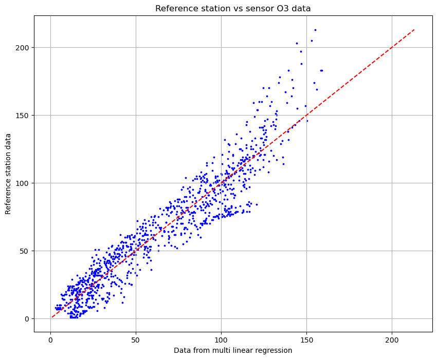
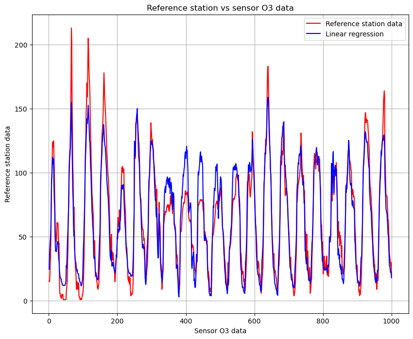
And this is the calibration of the signal:

If you are interested to the complete code, this is the repository where you can find it: Homework 3.

That’s all

The results highlight how well the model matches the values from the reference station, and show us a strong accuracy in the predictions. Thanks to the multi linear regression we verified how practical and useful this method can be.

The multi linear regression is a first step to go deep in the fascinating world of data science and machine learning. It can be applied in very different scenarios and it is the easiest approach when we need to combine multiple data to reach a final value. I hope this could be useful to you!

Thanks for reading!😃