Denoising data, which technique?

February 17, 2024 - 10 minutes

Summary

1. What is the experiment?
2. RMSE minimization
3. Gavish er al. Method

What is this experiment?

In this experiment I want to show you two different approaches that can be used to denoising a dataset. In these cases, the goal is to calculate the best low rank approximation of the data that allows us to obtain the best denoised dataset.

First of all, it’s important to say that these two techniques, RMSE minimization and Gavish et al. method, are used in different contexts. In the first case we have available a reference dataset that we can use to compare our results and try to get the best rank approximation. So we calculate the RMSE to achieve the lowest RMSE. In the second case, differently, we don’t use the reference dataset, but we will use a technique that allows us to establish which is the lowest rank approximation.

Ok, but can you explain better?

Yes, of course. The rank of a matrix is considered as the dimension of a vector space generated by the columns of the matrix. You’ll wonder which matrix. Well, in this case we have available the matrix of the dataset (then I explain how this matrix is composed) that contains all the data that we want to denoise.

SVD decomposition, what?

The SVD decomposition is a a factorization method used in algebra for data reduction, so from a large matrix, we can obtain a matrix with lower dimensions that still describes the same data. This is used, for instance, in the Principal Component Analysis (PCA) to get the effective rank of a matrix. This decomposition is used in order to change the coordinate system and try, therefore it allows to analyse the problem from a different point of view. This approach is used a lot for regression and in a plenty of machine learning techniques.

The powerful of this factorization is that we can apply the decomposition even if we have a non-square matrix, so, unlike by the Eigen Value Decomposition, we can use SVD with every matrix. More formally the SVD is defined:

where A is the matrix on which we want to get the decomposition:

• $U$ and $V$ are the orthonormal matrix, i.e. $U^T U = I$ and $V^T V = I$, and they are composed respectevely by columns called left and right singular verctors
• $\Sigma$ is the diagonal matrix composed by singular values

Singular vectors and singular values are analogous to eigenvectors and eigenvalues. Remember that eigenvectors represent the behavior of a matrix on specific directions, while eigenvalues define how much the matrix stretches or shrinks along those directions. Similarly, singular values describe how much certain directions are scaled (not necessarily orthogonal) by the matrix, and singular vectors represent those directions. This is very useful, as we’ll see.

# For further insights and evidence on these topics I recommend reading my post about the algebra used in machine learning or any algebra book. It is really interesting!

The low-rank approximation (Eckart-Young approximation)

As I said previously, the main goal of the experiment is to calculate the low-rank approximation of the dataset matrix, where k is the rank of the matrix. This technique is used in different cases:

• Compression data: a low-rank approximation return, as a result, a compressed version of the data. This is used for image compression, for instance. Assuming that $A$ is the matrix where each item represents a pixel of the image, we can use the low-rank approximation to reduce the number of pixel, but we guarantee that the image is understandable.
• Denoising: we clear up the signal by useless information that disrupts the signals. In this scenario, a low-rank approximation allows to get the true signal without the noise. Consequently, the matrix becomes more informative than its original form. This is what we want to do in this experiment.

In order to do the low-rank approximation we assume that the matrix $A$ has as dimension $n \times m$ (where n is the number of row and m the number of columns), so the rank r will be $r = min(n,m)$ (assuming that every row and column is linear independent between each other), so the low-rank approximation consists to find:

At the end of this operation we’ll get a matrix with rank $k$. Doesn’t sound too hard, isn’t it?

Let’s talk about the data

In this experiment, the dataset measures the $O_3$ levels in the air in a specific area. The dataset that we’ll use contains two different datasets:

• Reference Station dataset: it is the dataset of the values measured by the sensors in the station. These values are considered the most reliable.
• Sensors dataset: it is the dataset of the values measured by the Low Cost Sensors (LCSs)

The goal is to obtain the best approximation of the reference dataset using the MLR and SVR datasets. Now we’ll see how.

The data describe measurements from May 10th, 2017 to October 5th, 2017, and theoretically, the system takes new values every hour (24 measures in total). Not all days are complete, thus, those days were not considered for denoising.

For this project, like most code in machine learning, I used Python. The following libraries will be used:

import numpy as np # for algebric operations
import csv # for reading and writing CSV files
import matplotlib.pyplot as plt # for data visualization
from sklearn.metrics import r2_score # for calculating R-squared score

The following code show how I got only the full days:

import csv

sensor_data = "data-HW2.csv"

days_to_remove = []
with open(sensor_data, "r") as dataset_file:
    reader = csv.reader(dataset_file)
    dataset = list(reader)
    index = 0
    counter = 0
    days = 0
    current_date = "10/05/2017"
    diff = False
    for row in dataset:
        if index > 0: 
            date = row[0].split(' ')[0]

            if diff:
                if counter == 24:
                    days += 1
                else:
                    days_to_remove.append(current_date)

                counter = 1
                diff = False
                current_date = date

            if date == current_date:
                counter += 1
            else:
                diff = True

        index += 1

with open(sensor_data, "r") as dataset_file:
    reader = csv.reader(dataset_file)
    dataset = list(reader)
    index = 0
    for row in dataset:
        date = row[0].split(' ')[0]
        if not (date in days_to_remove):
            file = open("only-full-days.csv", "a")
            file.write(f"{str(row[0])}, {str(row[1])}, {str(row[2])}, {str(row[3])}\n")
            file.close()
        index +=1

This code will write in a new file called only-full-days.csv which contain all the full days in the dataset.

RMSE minimization

Now that we have the new CSV file, we can start with the RMSE minimization. First, let’s introduce how it works.

The RMSE (Root Mean Square Error) is a statistical index that helps understand errors and measures the average magnitude of errors in approximating the Reference Station data. It is calculated by taking the square root of the average of the squared differences between predicted and actual values. A lower RMSE indicates better accuracy of the model, resulting in better predictions. This is the formula:

Below is the Python code that I will use:

def calculate_rmse(X, Y):
    X, Y = np.array(X), np.array(Y)
    difference = X - Y
    squared_diff = difference**2
    mean_square_diff = np.mean(squared_diff)
    rmse = np.sqrt(mean_square_diff)
    print(f"RMSE = {rmse}")
    return rmse

In this experiment, I also want to evaluate the $R^2$ another very important index used to indicate how much of the variation of a dependent variable is explained by an independent variable in a regression model. Usually it is considered as a percentage and a value greater than or equal to 85% is considered good. This is the formula:

And this is the Python code that I will use:

def calculate_r2(X, Y):
    X, Y = np.array(X), np.array(Y)
    r2 = r2_score(X, Y)
    print(f"R2 = {r2}")
    return r2

In both of the previous functions, where $X$ and $Y$ are vectors.

Now, since the Sensors dataset contains data with different units of measure compared to the Reference Stations dataset, I need to show them in another way. The solution is the normalization of the data.

The normalization is an operation that consists to transform the data in order to have a mean $\mu = 0$ and a variance $\sigma^2=1$.

First of all, I calculate the average vector of all days of the reference dataset. I used this formula:

where $x_i$ are the vectors of reference dataset $X$ where each vector is composed by 24 values (one per hour), in my case $X=[x_1,...,x_M] \in \R^{D\times M}$ where $D=24$ and $M=104$. $\Psi$ represents the average set of data acquired by each sensor.

Let’s consider as $Y$ the matrix containing sensors data, on which we want to perform the normalization, and let’s say that $Y'$ is the normalized matrix. The normalization consists to subtract to each vector of $X$ the $\Psi$ vector, in this way I can calculate how much every vector of the dataset is far from the average vector. I use the following formula:

where $y_i$ is each vector of $Y$ matrix. I repeat the same operation also for the Reference Station matrix and I get the normalized matrix $X'$.

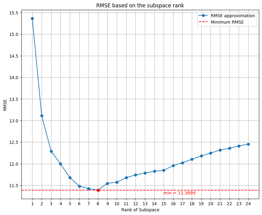
Now I calculate the approximation matrix. I don’t know which is the best low-rank approximation, so I calculate the RMSE for every rank and the result will be the rank with the lowest RMSE. In order to do this, I calculate the SVD decomposition on the normalized Reference Station matrix $X'$:

Then I use the following formula for the calculus:

where $U_k$ is the matrix of rank $k$ obtained by the SVD of the reference data, and $\hat{y_i}$ is the vector of the computation in the formula. At the end I build the $\widetilde{Y}$ matrix that is composed by the $\widetilde{y}$ vectors. Once I get the $\widetilde{Y}$ matrix I can calculate the RMSE value using as a reference the $X$ matrix. So I repeat the formula comparing every vector of $X$ matrix with the corresponding vector of the $\widetilde{Y}$ matrix.

This is the code that allows to get the new matrix:

def get_X_by_rank(REF, matrix, psi, rank):
    U, S, VT = np.linalg.svd(REF, full_matrices=False)
    U_k = U[:, :rank]

    new_matrix = np.empty((0,24))
    for vector in matrix.T:
        product = U_k@U_k.T@vector
        new_vector = psi + product
        new_matrix = np.vstack([new_matrix, new_vector])
    
    new_matrix = new_matrix.T
    return new_matrix

def getMatrix(dataset):
    X = np.empty((0, 24))

    index = 0
    for value in dataset:
        if index < 24*104:
            X = np.vstack([X, dataset[index:index+24]])
        else:
            break
        index+=24
    X=X.T
    return X

X = getMatrix(refer_dataset)
Y = getMatrix(sensorS_dataset)

ref_matrix = X

psi = np.mean(X, axis=1)

# normalization of sensors dataset
newY = np.empty((0, 24))
for y in Y.T:
    newY = np.vstack([newY, np.subtract(y, psi)])

Y = newY.T

# normalization of ref data
newX = np.empty((0, 24))
for x in X.T:
    newX = np.vstack([newX, np.subtract(x, psi)])

X = newX.T

ranks = []
rmse_values = []
min = 1000
rank_min = 0
for r in range(1, 25):
    newX = get_X_by_rank(X, Y, psi, r)
    rmse = calculate_rmse(ref_matrix, newX)
    if rmse < min:
        rank_min = r
        min = rmse
    ranks.append(r)
    rmse_values.append(rmse)

The result that I obtained is incredible, with the SVR dataset I got as best low-rank approximation 8:

This is the comparison with the initial dataset and the denoised datset of 5 days.

Before:

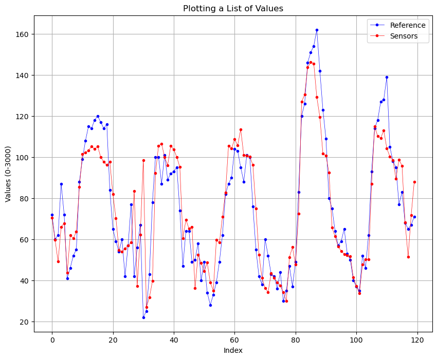
After:

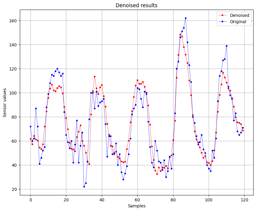
We can see that there is a slightly improvement of the quality of the signal, this is also confirmed by the RMSE values, where initially was of 13.424 and after the denoising is 11.3899. Also the $R^2$ is impoved, initially was of 0.8764 (87%) and now is 0.9110 (91%).

Gavish et al. method

Now I repeat the denoising of data using the Gavish et al method. With this method we don’t use the a reference dataset but we use just one dataset, then I will compare the results with the Reference Station dataset to check whether the obtained results are better or not. The main goal of this method is to try to find a low-rank approximation without use the Reference Station data.

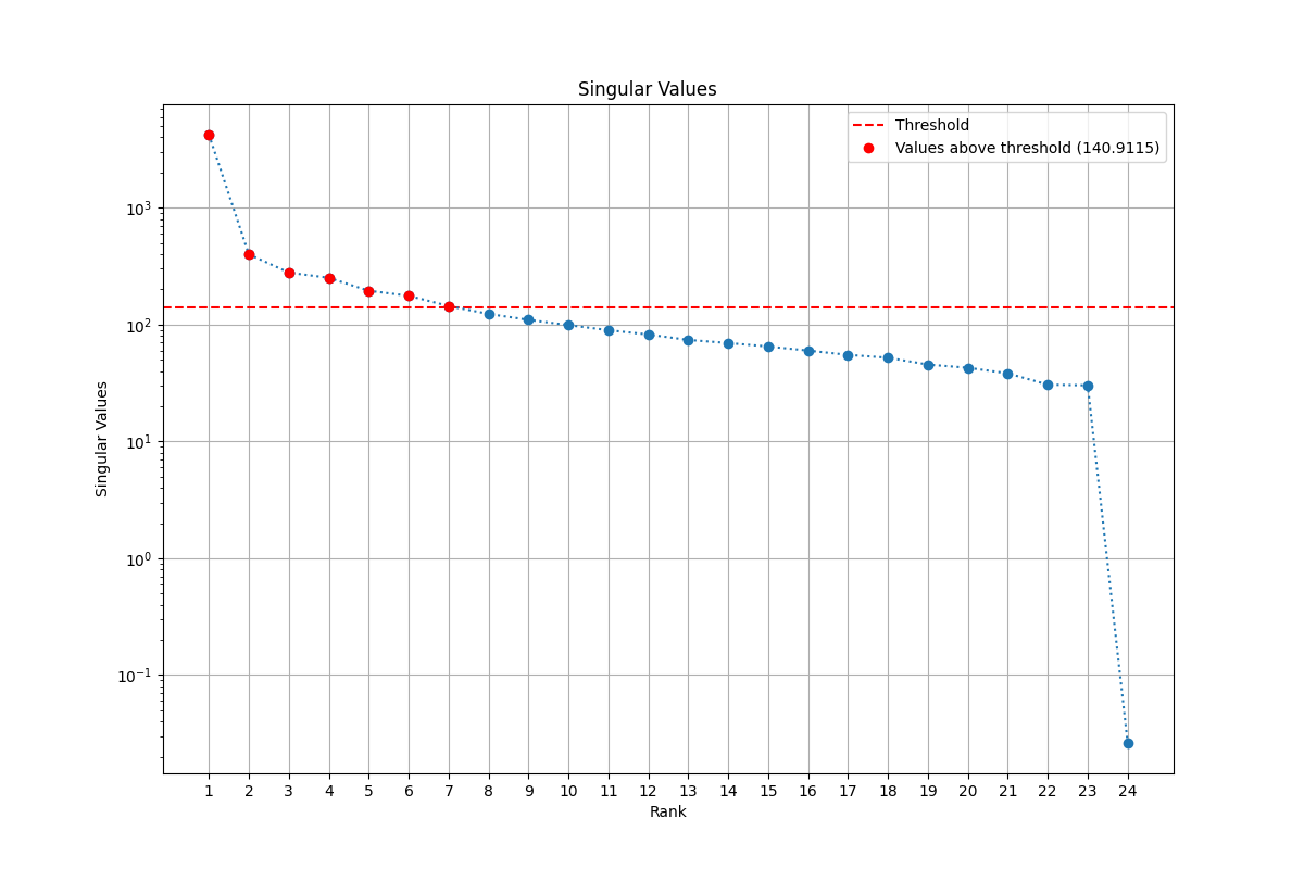
First of all I have to find the rank for the approximation. In order to do this, I find a threshold value. The threshold value is found by the following formula:

where $\beta=\frac{D}{M}=\frac{24}{104}$, $\sigma_{median}$ is the median of the singular values obtained by the SVD decomposition and $\omega$ is the following function:

Once the threshold value $\widetilde{\sigma}$ is found, I use the $\Sigma$ matrix calculated from the SVD decomposition in order to find the rank approximation. In fact the $\Sigma$ matrix contains on the diagonal the singular values in descending order. The minimum singular value above of the $\widetilde{\sigma}$ defines the rank for the approximation.

The code is the following:

Y = getMatrix(my_dataset)
U, S, VT = np.linalg.svd(Y)

median = np.median(S)
print(f"median = {median}")

beta = 24/104
omega = 0.56*(beta**3)-0.95*(beta**2)+1.82*beta+1.43
print(f"omega = {omega}")
sigma = omega*median
print(f"sigma = {sigma}")

rank = np.sum(S > sigma)
print(f"the rank is = {rank}")

Once we have the minimum rank, we can repeat the operation that we did in the low-rank approximation, but with some differences. In this case, since we have to denoise the data without use the Reference Station data, first I calculate the $\Psi$ vector using the Sensors dataset. Then we calculate the $\hat{y_i}$ subtracting $\Psi$ for each vector of the matrix of the dataset. These vectors will compose the normalized matrix. Then we calculate the $U$ matrix of the normalized matrix using the SVD. Finally we get the denoising vectors using the formula $\hat{y_i}=y_i-\Psi$ where $\Psi$, $U$ and $\hat{y_i}$ have just been calculated and we obtain $\widetilde{Y_i}$ that are the vectors of the denoised matrix.

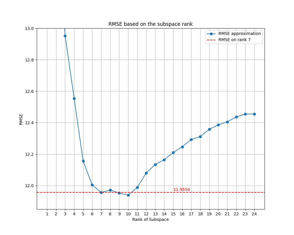
The result that I obtained for the low-rank approximation is 7. This is how I got it:

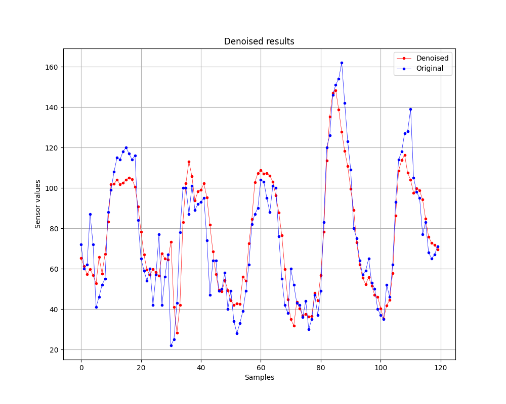
The result of $R^2$ is 0.9020 and the RMSE is is 11.9556. These results are quite good, as we can see in the picture:

Finally, I want to also show you the denoised result with this method:

We did it!

In these tests, we compared two different approaches to data denoising. In the first case we used Reference Station data, this method provides better results because we can compare the denoised dataset obtained with reliable data. Instead, with Gavish et al method, we used only one dataset and tried to denoise it without any comparison with the experimental data.

Although the first impression is that having the Reference Station data provides better results, the outcomes we obtained are quite similar between the two approaches. Even though having a lot of experimental data is the best way, however this is not always possible in practice, due to too high costs. Despite that, the results show that we can denoise data efficiently even without Reference Station data.

If you are interested to the complete code, I leave here my github repository where you can find it: Homework 2.

Thanks for reading!😃