Feedforward Neural Network: what it is

September 2, 2024 - 12 minutes

Summary

1. What is a FFNN?
2. Model
3. Neurons
4. Datasets
5. How the model works

Today, I want to discuss the Feedforward Neural Network, a class of artificial neural network models used in Machine Learning and Artificial Intelligence contextes. This model, also called Multi Layer Perceptron (MPL) is one of the simplest neural network models, but it is very good to understand how a neural network works. Let’s start with the basis.

FFNN an overview

Let’s start with a brief overview. A neural network is a collection of connected nodes, called neurons or perceptrons. Every neuron is a scalar function $f_i^{(L)}$ that evaluates each component of the vectorial function $f_i^{(L)}$. Neurons are collected by layers and the results produced by the neurons of a layer are sent to the neurons of the next layer.

The procedure of producing and passing data from a layer to the next one, continues until the final layer (output layer), which produces the final result. Based on the type of problem that the neural network solves, the outcome can be different. In general there are two types of problems:

• Classification problem: in this case, the outcome produced by the output layer is a label. It is used to define the nature or a description of the input. A popular application of this problem is, for instance, the images classification, where the model analyzes a picture and it is able to recognize the content in the picture.
• Regression problem: in this case, the outcome produced by the output layer is a numerical value. It is used to predict results based on historical data or to manipulate and combine the data in order to get meaningful results. Examples of this problem are applications that have to do with probability calculation and predictions.

In very simple words, the goal of a machine learning model is to try to determine a complex function that describes a pattern in the historical data. Once this function is calculated, it can be used to predict the outcomes starting from new data. It is important to say that the results provided by a machine learning model are not 100% correct, but they come from a probabilistic calculation.

Before delving into the different stages of the model functioning, I want to define some intrinsic characteristics of a neural network. Let’s see what they are.

Model

A neural network is composed of sets of neurons that communicate between them. This communication is not done randomly, but there is a specific structure that they follow. This structure is composed of different layers, each layer containing a set of functions, the so-called neurons or perceptrons. Each layer produces a set of results that are sent to the next layer. The layers can be categorized in different way:

• Input layer: this is the first layer, where the input data is read for the first time. The first layer has a number of input neurons equal to the number of features that we have in the dataset.
• Hidden layer: usually the hidden layers are several. Those layers are placed after the input layer and before the output layer. The number of neurons contained in these layers can be freely selected and it can be chosen based on the scenario that we want to evaluate.
• Output layer: this is the final layer. From this layer the forecasted features are yielded.

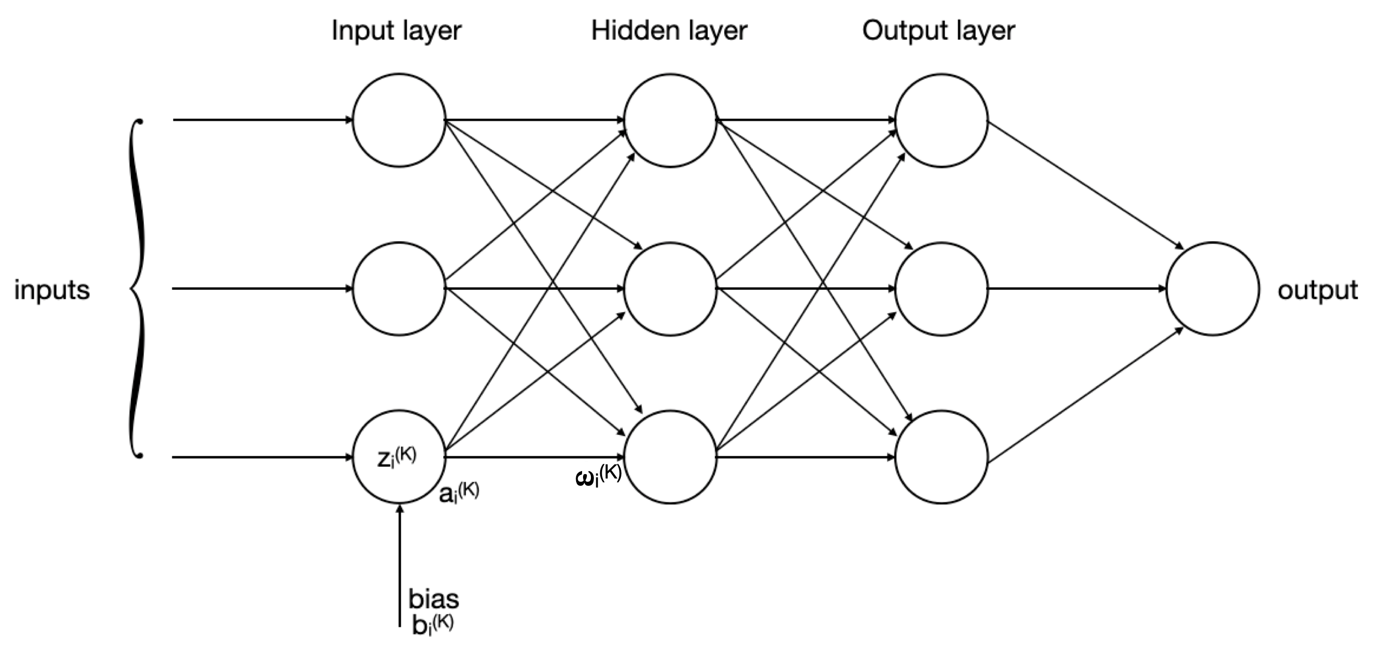
In the previous image, we can see that $z_i^{k}$ is the weighted sum of the inputs, $b_i^{k}$ the bias added to the weighted sum, $a_i^{k}$ the activation function applied by the neuron i-th neuron of the k-th layer and $\omega_i^{k}$ is the weight of the of the connection between the i-th neuron in the k-th layer and the j-th neuron in the (k+1)-th layer. Now, I am going to explain better what every parameter represents.

Neurons

As we said, the neurons are functions which are composed by different parameters: internal parameters and hyperparameters.

Internal Parameters

These parameters are located within the model. These values are adjusted by the model during training in order to minimize the loss function. They allow to find the relationship and the pattern within input data. In FFNN, the parameters are the following:

• Weights: the weights are parameters that control the strength of the connection between two neurons. The higher the weight is, the stronger the influence of the connection on the output is. Each connection between neurons has an associated weight. For every neuron j in the same layer k, the input from the neuron i in the previous layer is multiplied by the weight w_ij that there is on the connection. x_i is the value of the input in the neuron and the total input to neuron j is the weighted sum of all inputs from the previous layer:

  $$z_i^{(k)} = \displaystyle\sum_{j}^{h_{k-1}} \omega_{ji} x_{i}$$

  This is the first operation applied to the input by the neurons.

• Biases: they are additional parameters that are added to the weighted sum calculated before:

  $$z_i^{(k)} = \displaystyle\sum_{j}^{h_{k-1}} \omega_{ji} x_{i} + b_j$$

  The biases are not influenced by the previous layer. They essentially act as an offset for the activation of the neuron, and they allow the model to capture patterns in the data. The bias unit guarantees that even when all the inputs are zeros there will still be an activation in the neuron.

• Logits: they refer to mathematical linear transformation applied to the vector of raw, unnormalized predictions generated by the last layer of a neural network before it is passed through an activation function. This is often used in classification task.

• Activation: it is the function used to activate neurons during the process. The activation function introduces non-linearity into the model, allowing the neural network to learn complex patterns in the data. There are different activation function, these are the most populars:

  • ReLU:

    $${\displaystyle ReLU(x)={\frac {x+|x|}{2}}={\begin{cases}x&{\text{if }}x>0,\\0&{\text{otherwise}},\end{cases}}}$$

  • Sigmoid:

    $$f(x) = \frac{1}{1 + e^{-x}}$$

  • Softmax:

    $$f(x_i) = \frac{e^{x_i}}{\sum_{j=1}^{n} e^{x_j}}$$

    for $i = 1, \dots, n$

  • Hyperbolic Tangent (tanh):

    $$f(x) = \tanh(x) = \frac{e^{x} - e^{-x}}{e^{x} + e^{-x}}$$

Hyperparameters

These parameters regard the way to train the model. They can be considered as external configurations of the model set before that the training process begins. The hyperparameters control the overall behavior of the model. These kind of parameters are:

• Learning rate: it is a hyperparameter that controls how much the weights of the model are adjusted with respect to the loss gradient during each update. Essentially, it determines the step size at each iteration while moving toward a minimum of the loss function. If the learning rate is too low, the model takes too long to achieve the minimum, but if its value is too high, the model tends to oscillate and never reach the optimal value.

  An example of an optimization algorithm used to minimize the loss function is Stochastic Gradient Descent (SGD). At each iteration, the model parameters are updated as follows:

  $$\Theta^{(t+1)}=\Theta^{(t)}-h\nabla_{\Theta}J(\Theta^{(t)})$$

  where $\Theta^{(t)}$ is the parameter used in the cost function at iteration $t$, $J(\Theta^{(t)})$ is the gradient, and $h$ is the learning rate.

• Number of neurons for each layer: it determines the capacity of the model. More neurons allow the network to capture complex patterns in the data, but this could potentially lead to the overfitting case. On the other hand, using too few neurons leads to the underfitting case.

• Number of epochs: one epoch is one complete pass through the entire training dataset. The number of epochs refers to the number of iterations that the model works through the whole training set, during the training stage. Even in this case, too many epochs leads to overfitting, as well, too few epochs leads to underfitting.

Datasets

Let’s consider that we have available a lot of historical data about a specific phenomenon. We want to exploit those data in order to build a model that is able to make a prediction regarding that event. So, let’s see how it is done.

The first thing to do is to split the data in different sets:

• Training set: it is the largest dataset. It contains the historical data on which the model that we are building bases the understanding of the relationship and pattern within the data.
• Validation set: it is the remaining part of the available data. This dataset is used to check if the model has understood well or not the patterns within the data, so it allows to evaluate the quality of the model.
• Testing set: it is the set that represents new data. This dataset is used to test the performance of the model after it has been trained and fine-tuned using the training and validation sets.

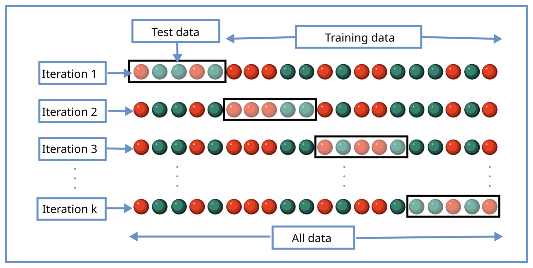
This method to split the data and train and test the model with different datasets is called cross-validation. Cross validation is a very used technique in machine learning to evaluate the performance of a model with unseen data. The process to split the data in different sets is repeated multiple times, in this way the sets built are different and the result of the validation stages are averaged in order to produce a robust model. With this method we can avoid overfitting.

# I have already talked about underfitting and overfitting problems in this post

Now, let’s see in detail how the above defined datasets are used.

How the model works

The principle of the neural network working is intuitive but also very interesting. It consists in three stages:

1. Training: this is the first stage and it indicates the phase where the model learns how to predict the data. The idea is to teach the model, as you do with children, when a behavior is right and when it is wrong. The difference is that here we don’t need to talk with a kid, but the model “just” fixes the internal parameters in order that it can learn how to predict a correct answer. The processes that allow to calculate and assign the values to the parameters are optimization operations, such as the gradient descent, where the goal is to minimize the loss function. The training requires a lot of data, so that the precision and the quality of the network improves. It can be done in two ways:

   • Supervised learning: in this case there are already some solutions to a problem. The training consists of passing the inputs of which we already have the correct outcome and trying the model in order that it can predict the wanted result. If we have a classification problem we need different datasets, one for each possible outcome; if we have a regression problem, we need a lot of historical data that match with several possible results. The network training consists of checking at the end of every iteration (epoch) if the outcome provided by the network matches with the correct output. The model uses a method to minimize the error between the true value and the predicted value and based on that it fixes the internal parameters in order to match the input with the corresponding output.
   • Unsupervised learning: in this case we don’t have available outcomes starting from the input yet. The model has to execute some preprocessing operation in order to identify some patterns in the data and figure out the relationship between input data and solution. This kind of operations includes Principal Component Analysis (PCA), autoencoders and clustering operations.

2. Validation: after training the model, the next step is to validate the model. In this stage we are going to check whether the model has understood correctly the relationship between the data during the training. This step is very important since it allows checking the performance by changing the hyperparameters. The hyperparameters are tuned in order to choose the best configuration of the model and avoid both underfitting and overfitting. This allows them to set a checkpoint in order to see how the model can perform with data different from the training set. If the model acts well with the validation set, most likely the quality of the model is good, and it can be used with data completely new. If the model provides bad results with the validation set, then it is recommended to change the hyperparameters and try a different configuration.

3. Testing: this is the final test, it consists of executing the model with data completely new. We say that this evaluation is unbiased, since the data are not taken from a known dataset where there can be residues of patterns of the historical dataset, but the data comes from a different source. This is the final step. In the testing, we can obtain the final performance metrics that allows to understand the quality of the model and understand how reliable the model is. Here, we can observe how good the model is by studying the bias-variance trade-off, to avoid overfitting. If the model is able to produce correct results in this stage, the model is done and you have done a great work.

Note that in this kind of machine learning problems, there is not any specific way to find the best model. The only way is to try with several combinations of the model and adjust the hyperparameters in order to get a result and calculate the values of statistical indexes such as RMSE or R$^2$. The one with the best values will be the final model.

I hope this brief introduction on the Feedforward Neural Network would have been useful, I will base the next posts about the FFNN on this, stay tuned! 😀