Underfitting and overfitting: an overview

August 1, 2024 - 7 minutes

Summary

1. What is the experiment?
2. Approximation and estimation error
3. Underfitting and overfitting
4. Bias-Variance trade-off

Introduction

In data science, especially in machine learning techniques, like regressions and unsupervised methods, it is really important to choose which parameters to consider and how to set those values. This is very challenging, specially because in some implementations the parameters are several and the possible combinations are a fair amount.

As we could think, the more we increase the number of the hyperparameters, the more the accuracy and the quality of the prediction is higher. Unfortunately, this is not true. This problem can lead toward two different non-desired situations: underfitting and overfitting.

Let’s take an example. Assume that we are using linear regression. We suppose that the linear model is correct so there is a true linear relationship between $X$ and $Y$, therefore the error is equal to zero:

However, in our example we have a very large number of hyperparameters to predict, but we only have available a limited number of samples. Let’s say 100 hyperparameters and 110 samples.

This problem implies a minimization problem that can be solved using the ridge linear regression. The cost function can be written as follows:

where $\lambda$ is a hyperparameter that controls the introduction of the penalization $\theta$ components.

Approximation and estimation errors

In the regression methods, there are two important different errors to take into account for a better understanding of the machine learning models.

We agree that a good prediction of the $y$ function represents a good model, however it is not possible to obtain a perfect prediction because of the probabilistic nature of the model. The model will try to predict and approximate the function $f$ that is a function of the class $F$, i.e. $f \in F$.

Hence, we can define two kind of errors:

• Approximation error: the difference that we obtain from the true function and the best possible approximation that the model can provide.
• Estimation error: the difference between the best possible model and the parameters estimated from the training set.

For every machine learning problem, if we have available a training set (TS) for the training of the model, there is always a trade-off between two terms. If our model uses a rich class of $F$, it will yield a greater estimation error with a smaller approximation error. On the other hand, if our model uses a very little class of $F$, it will yield a greater approximation error with a smaller estimation error. It is very important to balance the size of the class $F$ in the model to ensure to not go from one extreme to the other.

Here we can se a clear example of very low approximation error but large estimation error:

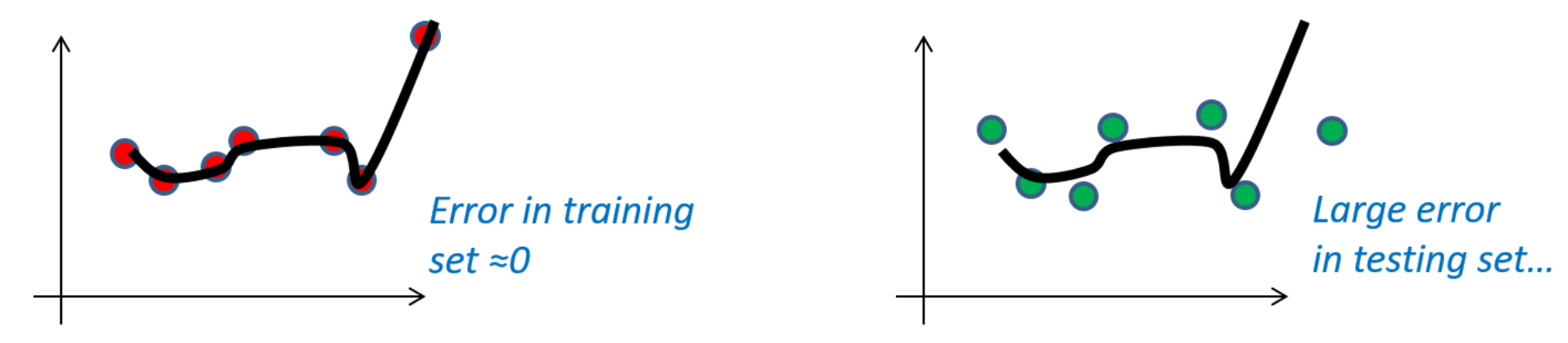
As we can see in the picture, since the error is equal to zero, if we set $\lambda = 0$ this leads to a very low approximation error but a higher estimation error.

Here we can already understand the main idea between underfitting and overfitting.

Underfitting and overfitting

Underfitting

These are the two situations that we want to avoid. Underfitting describes the situation in which we are using a too simple machine learning model, so we are considering a too large set $F$, in other words, too many possibilities.

For instance, if we use a linear regression model of the form: $\phi^t(X) = (1,X)$ we will have probably an underfitting problem, as our estimation of $f$ will have necessarily the form:

This leads to not including the good approximation of the optimal function $f$. In this way we are trying to predict the actual function with just two parameters, and this could be too approximative, therefore the approximation error is large.

Overfitting

On the other hand, we have also the overfitting. It describes the situation where we are using too many parameters, so the model is too complex. In this case the set $F$ is too small and it allows us to find just a few possible functions. Moreover, the training set is too small and it does not allow us to make a good estimation of the $f$ that we are looking for.

If we use a linear regression model of the form: $\phi^t(X) = (1,X, X^2, X^3,...,X^{10})$ we can potentially find a very good estimation of the true solution, in other words, our approximation error is very small. But if we assume that the training set is small, the model will fit exactly the training set. This means that in every other case, the solution will provide more or less the same shape of the function.

Here, the estimation error is large. Overfitting is less intuitive than underfitting, as it is easy to believe that complex models are always better than simpler models.

Bias-Variance trade-off

Now, let’s talk about something interesting. From the previous definitions, we defined some errors and some situations that we want to avoid. The errors in statistical models can be formulated in different ways, but one of the most used index errors is MSE (Mean Squared Error). This indicator measures the average difference between values predicted by the model and the actual values. The formula is the following:

This index is really important, since it describes the accuracy of the model.

Another interesting way to write the index is this:

# I don't show the proof of this formula, for further information I recommend this paper

Each factor can be decomposed and written in this way:

Where we can define $f_T$ as the true function on a dataset $T$ that approximates $f(x)$.

In the formula we have three components:

• Bias: measures the difference between the predicted value and the true function. This can be considered as the error that the model commits based on the training done previously.
• Variance: measures the variance of the model’s solution. It defines how much the predictions would change if we use a different training.
• Irreducible error ($\sigma^2$): is the noise due to the data that we have available. It cannot be reduced because it depends on the dataset and not by the quality of the model. It changes based on the randomness of the data.

Now that we have some definitions, let’s take the following picture, that is very significant.

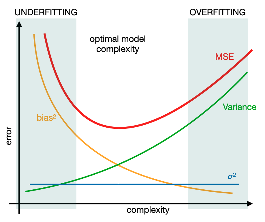
From this graph we can do some assumptions:

If the complexity is low

The bias is very high and the variance is very low. In general the error is high because of the bias component, therefore a high bias increases the approximation error because the model is too simple to predict the correct function. This is the underfitting.

If the complexity is high

The variance increases and the bias decreases. The error that we can find here is due to the variance, therefore a high variance increases the estimation error because the function calculated by the model is too correlated to the training set used to train the model. This is overfitting.

Final considerations

The best solution that we can achieve, as we can see, is in the middle. A good model should not be too simple to avoid the underfitting but at the same time it should not be too complex in order to avoid the overfitting. How can we find the best middle way? The simplest and the most effective solution is to try with several tests and verify in which conditions we can achieve the smaller error, as I did in the previous in the denoising post. In general, in machine learning, there is not a way to find the best model without testing. In addition, in some cases the error of the model keeps pretty high even though we built a very good model. This is due to the size and the quality of the dataset that is crucial for determining the level of the error.

Thanks for the attention! 😃